Most of the time, mechanical systems behave exactly how you expect them to: you excite a mode, it rings down, and motion fades away. However, in systems with extremely low dissipation, that idea, while true, is more complicated to model. Specifically, a clean oscillator turns into something richer and harder to reason about. Currently, in the Quantum Atom Optics group at Northwestern, I’m studying the dynamics of a particular type of system: diamagnetically levitated quartz particles. These are ultra-high-Q mechanical oscillators that can ring for days. Over thse large time scales, frequencies start drifting in ways that don’t fit a simple exponential decay, so I needed a way to classify modes (6 modes, 1 for each degree of freedom). Here’s a related paper I helped write on the subject for a deeper explanation.
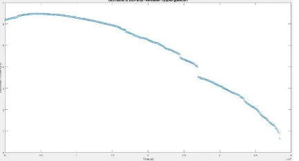 Figure 1: Example of a ‘quadratic’ decay (not exponential) of energy in a single mode
I also wanted a way to let the data speak for it self and automatically surface when something new in the behavior of the particle was happening, without having to spend time hardcoding thresholds. I decided to apply the skills learned in my machine learning class (EE375) to help me tackle this problem, and the result is the pipeline described in this post! Happy reading!
Table of Contents
Open Table of Contents
Introduction
The goal of this project is to build a data-driven pipeline that can automatically surface these behaviors. Rather than hand-labeling events or tuning thresholds, I wanted a workflow that starts from raw displacement data, extracts physically meaningful features, and then lets structure emerge naturally using unsupervised machine learning.
Experimental Context
Without revealing too much about the experimental procedure (paper coming out soon!), I’ll try to put the data in context of the work. Motion of a particle is read out using a quadrant photodiode analysis of pixel data (from a camera recording, 30 fps), which provides a time-domain displacement signal along orthogonal axes. Because the particle has extremely low dissipation, its mechanical modes ring for long times, making it an ideal platform for studying weak nonlinear effects. In practice, the data acquisition is broken into many short recordings. Each recording coresponds to a time-domain signal, and from this, a spectrogram, but gaps between the recordings exist. Thus, any meaningful analysis has to take into consideration a discontinuous dataset.
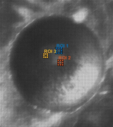 Figure 2: Example levitaded cube with assymetries in both trap (magnetic potential well) and geometry of cube that contribute to nonlinearities.
Raw Data
Each recording produces a spectrogram with several visible peaks corresponding to various mechanical modes (and their harmonics). The modes were matched to the physics of the objects from theoretical estimates (as outlined in this paper). The spectrogram segments were stitched into a long continuous dataset, where each segment is rescaled onto a standardized time window and shifted into place using known delays between recordings.
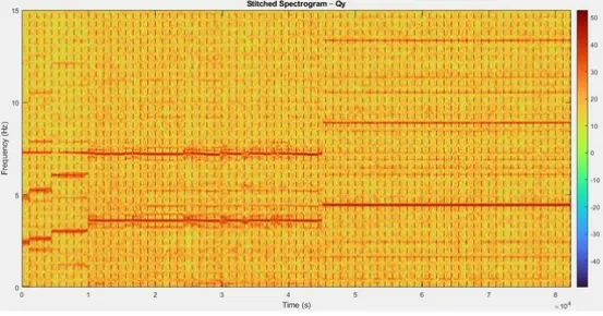 Figure 3: Spectrogram of a single instance of time-domain signal
Tracking Mechanical Modes
Once the stitched spectrogram is available, the next challenge is tracking the individual mechancial modes over time. However, simple peak picking only works if the modes are well-seperated and stationary. In long experiments, modes can drift, cross, or recurrently exchange amplitude (FPUT behavior). In these cases, naive peak selection can jump between the modes or lose track of them entirely.
To address this, I implemented a cost-based mode tracking algorithm. At each time slice of teh spectrogram, all candidate peaks are indentified and assigned a cost relative to the previous frequency of a given mode:
Here, is the candidate frequency, is the previous tracked frequency, and is the normalized peak amplitude. This formulation favors the continuty in frequency while still allowing strong peaks to pyll the tracker when real mode interactions occur. Additional constraints are set in code to limit the maxiumum allowed frequency jump per time step.
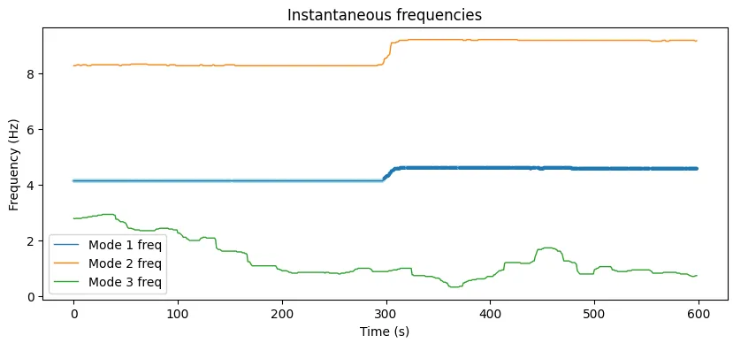 Figure 4: Frequencies of mdoes drift over time
Adaptive Hilbert-Based Feature Extraction
Spectrogram amplitudes alone do not capture the dynamics of a system. Specifically, I need to extract the instantaneous amplitude, frequency, and phase information using an adapative (sliding window) Hilbert transform appraoch. For each tracked mode, I applied a narrow bandpass filter centered on the mode’s instantaneous frequency, which is updated dynamically as the frequency drifts. Sliding a window across the time-domain signal, I computed the analytic signal and extracted
- amplitude envelopes
- instantaneous frequencies
- relative phase trajectories
The relative phases between mode pairs are also computed to analyze phase locking and nonlinear coupling behavior.
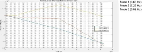 Figure 5: Relative phase differences between each of the 3 modes.
From Signals to Feature Vectors & Learning
At this point, each time index can be represented as freature vector containing
- tracked mode frequnecies,
- hilbert amplitude envelopes
- hilbert instantaneous freqeuencies
- pairwise relative phases
All the features are resampled then onto a common time base and normalized. More importantly, every feature as a distinct physical interpretation! Yay!
Unspervised Learning
There are no ground truth labels for linear vs nonlinear behavior in this system, since transitions are often gradual or ambiguous (at least to me). Unspervised learning provides a way to ask the question: do different parts of the experiment look dynamically different from one another?
UMAP: Strucuture in the Dynamics
To visualize the structure of the feature space, I use UMAP (Uniform Manifold Approximation and Projection). UMAP preserves local neighborhood relationships, making it well0suited for identifying distinct dynamical regimes. When the feature vectors are embedded into two dimensions, the data seperates into distinct clusters, indicating that the system occupies qualitatively distinct states over time. To illustrate this, I used a recording in which there was an obvious ‘nonlinearity’ due to a pulsive artifact (bumping into the setup) and attempted to seperate a ‘linear’ regime from a the noise source.
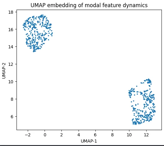 Figure 6: UMAP embedding in two dimensional space
Clustering Dynamical Regimes
To formalize these groupings, I applied HDBSCAN, a density based clustering algorithm. HDBSCAN indentifies clusters of arbitrary shapes and labeles low-density regions as noise, which may correspond to transition periods between regimes. The resulting clusters align closely with visible changes in frequency drift, amplitude envelopes, and phase behavior.
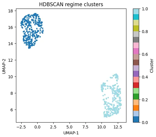 Figure 7: Clustering (quite obviously correct) shows two distinct clusters, each corresponding to a different dynamical regime.
Back to Physics
The cluster boundaries actually correspond to physical events: frequency jumps, energy redistribution between modes, and phase reorganizatoin. PCA analysis actually shows that these events dominate some specific principle components, which can provide an interpreatable ‘linear’ and ‘nonlinear’ summary of dyanmics (similar to the sine sweep demodulation technique I described here). It seems that these results suggest that the system undergoes transitions between weakly coupled and strongly coupled regimes, and the observed behavior seems consistent with nonlinear mode coupling and energy exchange reminscent of Fermi-Pasta-Ulam-Tsingou type dynamics in low-loss mechanical systems.
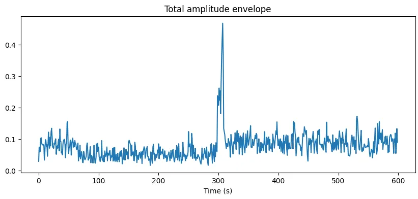 Figure 8: Total energy amplitude (spike corresponds to pulsive noise source)
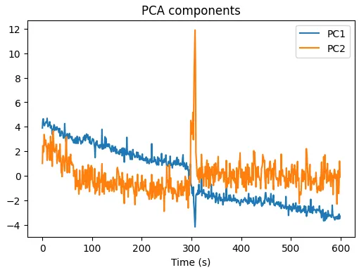 Figure 9: Extracted PCA amplitude components corresponding to a linear (blue) decaying behavior as well as a pulsive noise artifact (orange).
I had a lot of fun learning about the different ML techniques commonly used in mode classification and learned a lot about relevant feature extraction and embeddings!