Sine Sweep Deconvolution

Table of Contents

Motivation

In the Northwestern Haptics Group, I’m attempting to characterize the lateral dynamic compliance and viscoelastic parameters of the fingepad in frequencies relevant to touch, which range from 30 to around 350 Hz.

In many systems, we provide an excitation that resembles an impulse (such as striking a baseball bat with a hammer). However, exciting the finger with a sharp impulse is not very practical, since it can be noisy, painful, and provide low SNR.

Instead, a common technique is to use a sine sweep method (linear or exponential), originally developed for acoustics, to obtain clean and artifact-free impulse responses. These sweeps spread energy over time, then mathematically repack it into an IR - while allowing for clean seperation of nonlinear distortion (harmonics) from the linear response. This information is adapted from this paper.

System Models and Signals

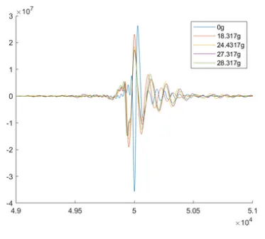
In my setup, I’m actuating a carbon fiber pin that indents into my finger, and a voice coil actuates the pin in a lateral motion. My input signal is the force (which I approximate by multiplying the force factor with the current going through the coil), and the output is pin displacement (scaled from LDV). We want to find the IRs of various setups (finger placement, indendation depth, orientation of finger, etc.). Here are some actual outputs:

However, the technique can be used to resolve IRs for any system that can be reasonably approximated as LTI for the duration of the sweep, with mild time variance and nonlinearity (ESS is pretty robust to both in practice).

Exponential Sweep

Let the drive signal be the exponential sweep $x(t)$ of duration $T$, starting at $\omega_1 = 2\pi f_1$ and ending at $\omega_2 = 2\pi f_2$:

The instantaneous frequency is

Because $\omega(t)$ grows exponentially, low frequencies are excited for longer (higher SNR at low $f$), while high frequencies sweep quickly. The resulting spectrum is “pink” (about $-3 \,\text{dB}$/octave), so the inverse filter must compensate by $+3 \,\text{dB}$/octave.

Aperiodic Deconvolution and Inverse Filter

We want the system’s IR $h(t)$:

where $y(t)$ is the measured output (finger displacement) and $f(t)$ is the inverse filter.

We take advantage of the following:

1. Aperiodic convolution (not circular), avoiding wrap-around artifacts.
2. Time-Reversal Mirror (TRM): take the time-reverse of the sweep and apply amplitude correction.

Because the sweep has a pink spectrum, the inverse filter amplitude must grow $\propto +3 \,\text{dB}$/oct. Thus:

with $K = T / \ln(f_2/f_1)$.

When $y(t)$ is convolved with $f(t)$:

• The linear response collapses into a sharp peak (delayed by $T$).
• The $k$-th harmonic distortion collapses into earlier peaks (time-separated from the main IR).

Pre-ringing and Bandwidth

If you taper the sweep (fade-out) or truncate bandwidth, the recovered IR looks like a sinc with oscillatory pre-ringing.

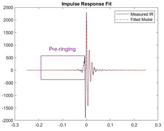
Fixes:

• Extend the sweep to Nyquist ($f = f_s/2$), then cut at the last zero-crossing.
• Avoid fade-outs; use only a minimal fade-in.
• For low-frequency ringing (from analog chains), apply a Kirkeby compacting inverse (see below).

Frequency-domain inversion (Kirkeby filter)

Given a measured IR $h(t)$, compute its FFT:

Then build a regularized inverse filter:

where $\varepsilon(f)$ is small inside the sweep band, larger outside.

Inverse transform:

This compacts the IR, reducing pre-ringing and whitening the response.

Practical Usage

Pulsive noise during sweepa

In some cases, there may be pulsive artifacts (like a tool drop). These are described can be described as a broadband click, and they deconvolve into descending sweep artifacts.

The best way to remove these is is to compute the instantaneous frequency at the click time click time $t_c$,

then apply a narrow band-pass filter around $f_\text{inst}(t_c)$ before deconvolution.

Clock Mismatches

If playback and recording clocks drift, the IR skews in the time-frequency plane. There are two fixes to this:

• With reference: Kirkeby inverse to correct delay vs frequency.
• Without reference: stretch the inverse sweep by the measured skew amount before deconvolution.

Averaging

It is good practice not to average many short sweeps, as it underestimates the high-frequency tails. Instead, it is recommended to use one long sweeps, and if repeats are necessary (example, skin varies from person to person in my application), average in the frequency domain.

where $G_{LR}$ is the cross-spectrum and $G_{LL}$ the auto-spectrum.

Basic Example

Here’s a basic example of what a deconvolution and seperation of linear IR from its harmonics could look like:

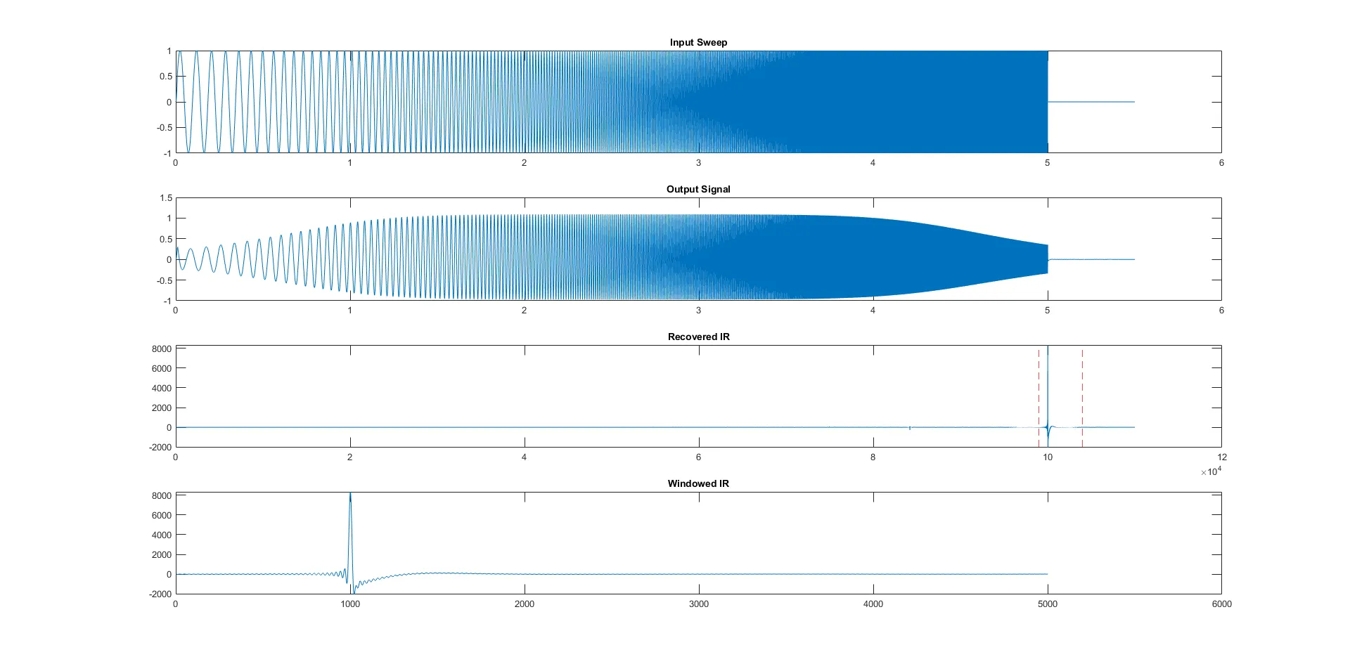
clear; clc; close all;

fs = 20000; T = 5; f1 = 10; f2 = 800; pad = 0.5;

t  = (0:1/fs:T)';
K  = T / log(f2/f1);
phi = 2*pi*f1*K*(exp(t/K)-1);
x   = sin(phi);
x   = [x; zeros(round(pad*fs),1)];
t   = (0:numel(x)-1)'/fs;

fade = round(0.01*fs);
x(1:fade) = x(1:fade).*linspace(0,1,fade)';

wCorr  = exp((0:1/fs:T)'/K);
f_inv  = flipud(sin(phi)) ./ wCorr;
f_inv  = [f_inv; zeros(round(pad*fs),1)];

[b,a] = butter(2, [20 500]/(fs/2), 'bandpass');
y_lin = filter(b,a,x);
y = y_lin + 0.06*(y_lin.^2) + 0.03*(y_lin.^3) + 2e-4*randn(size(y_lin));

h_rec = fftfilt(f_inv, y);

[~, i0] = max(abs(h_rec));
i1 = max(1, i0 - round(0.05*fs));
i2 = min(numel(h_rec), i0 + round(0.2*fs));
h_win = h_rec(i1:i2);

subplot(4,1,1);
plot(t, x); title('Input Sweep');

subplot(4,1,2);
plot(t, y); title('Output Signal');

subplot(4,1,3);
plot(h_rec); title('Recovered IR'); hold on
xline(i1,'r--'); xline(i2,'r--');

subplot(4,1,4);
plot(h_win); title('Windowed IR');