Streaming FM Radio

Table of Contents

Introduction

This is a writeup of my final project for CE387 (Real-Time Digital Systems Design and Verification with FPGAs), for which my partner, Zach Tey, and I designed and verified a digital streaming FM stereo receiver implemented in SystemVerilog. The goal of the system is to process raw complex baseband I/Q samples and reconstruct stereo audio in real time using a modular, hardware-efficient architecture.

Modern communication systems increasingly rely on DSP techniques to replace traditional analog radio circuits. The input to the system consists of complex I/Q samples obtained from a software-defined radio (SDR) front-end (provided by our professor). These samples encode the FM-modulated broadcast signal in baseband form. The receiver must extract the instantaneous frequency information, separate the multiplexed stereo components, and reconstruct the left and right audio channels. This requires implementing several key signal processing blocks, including finite impulse response (FIR) filters, a quadrature FM demodulator, frequency translation stages, and de-emphasis filtering.

A major focus of this project is the translation of algorithmic DSP concepts into a fixed-point, streaming hardware implementation. All modules are designed using a valid-ready handshake interface, allowing continuous data flow while accomodating for any processing latencies.

In addition to design, we verified the outputs to a ‘golden-reference’ model, which was generated by C/MATLAB. To do this, we built a Universal Verification Methodology (UVM) environment to verify the entire pipeline after verifying individual stages. The entire source code is available here.

FM Radio Theory

Frequency Modulation (FM) is a method of encoding information in a carrier signal by varying its instantaneous frequency according to an input signal. Unlike amplitude modulation, where information is carried in the signal magnitude, FM keeps the amplitude constant and instead encodes the message in the rate of change of phase. The transmitted signal can be written as

where $f_c$ is the carrier frequency, $m(t)$ is the message signal, and $k_f$ determines the frequency deviation. In broadcast FM, the carrier frequency lies in the range of 88—108 MHz, while the audio signal occupies a much lower frequency range (typically up to 15 kHz). Modulation allows this low-frequency signal to be transmitted efficiently using a high-frequency carrier.

In a digital receiver, the incoming RF signal is downconverted to baseband and represented as complex in-phase (I) and quadrature (Q) samples. These samples capture both the amplitude and phase of the signal. The key information in FM lies in how the phase changes over time, so the goal of demodulation is to estimate the derivative of the phase. Given I/Q samples, the instantaneous phase is

and the audio signal is proportional to the phase difference

In practice, this is computed using algebraic approximations that avoid expensive trigonometric operations. A commonly used expression is

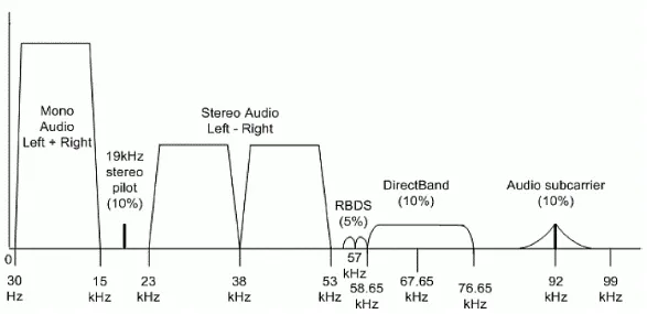
FM stereo transmission includes additional structure beyond the baseband audio. The transmitted signal consists of three main components: the mono signal $(L+R)$, a pilot tone at 19 kHz, and a stereo difference signal $(L-R)$ modulated onto a 38 kHz subcarrier. The mono component allows compatibility with legacy receivers, while the stereo information is encoded in the higher-frequency components. The pilot tone serves as a reference that allows the receiver to reconstruct the 38 kHz carrier needed to demodulate the $(L-R)$ signal.

To recover stereo audio, the receiver first extracts the mono component using a low-pass filter. The pilot tone is isolated using a band-pass filter and then squared to generate a 38 kHz signal. This reconstructed carrier is used to mix the $(L-R)$ band back down to baseband. Finally, the left and right audio channels are reconstructed using

Additional filtering, such as de-emphasis, is applied to compensate for the pre-emphasis used during transmission, which improves noise performance at higher frequencies.

System Architecture

Overview

The system is composed of several parameterized RTL modules connected in a streaming pipeline. Each module is designed to operate on fixed-point data using a valid-ready interface, which allows for sample processing while handling variable internal latencies.

The overall architecture follows the standard FM receiver structure: channel filtering, demodulation, stereo extraction, and reconstruction of left and right audio signals.

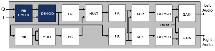
The top-level integration is handled by the fm_radio and fm_radio_top modules. The fm_radio module instantiates and connects all DSP blocks, including FIR filters, demodulation, multiplier stages, and stereo reconstruction logic. The fm_radio_top module serves as the interface between the external byte stream input and the internal fixed-point pipeline, handling I/Q reconstruction and final audio output formatting. These modules are primarily structural, with minimal internal logic, and rely on FIFO-based buffering to manage timing between stages.

The multiplier block is another core component and is reused across multiple parts of the pipeline, particularly in stereo decoding. It performs fixed-point multiplication followed by scaling and saturation. The scaling is implemented using an arithmetic right shift, but to ensure truncation toward zero (matching the C reference), a bias is added to negative values before shifting. This prevents systematic errors that would otherwise accumulate across the pipeline. The multiplier is used for operations such as squaring the pilot tone to generate a 38 kHz carrier and mixing the L−R signal back to baseband. Because multiplication corresponds to frequency shifting in the time domain, this block plays a central role in reconstructing stereo information.

The IIR module is used for de-emphasis filtering in the audio stage. Unlike the FIR filter, which relies only on current and past inputs, the IIR filter also uses past outputs to implement a recursive structure. This allows it to achieve a desired frequency response with fewer coefficients, reducing hardware cost. The implementation stores previous input and output samples in registers and computes the output using a combination of feedforward and feedback terms. Fixed-point scaling and saturation are applied to maintain stability and prevent overflow. The recursive nature of the filter requires careful handling of timing to ensure correct data dependencies between cycles. The add_sub module performs stereo reconstruction by combining the L+R and L−R signals. It computes the left channel as (L+R + L−R)/2 and the right channel as (L+R − L−R)/2. The implementation consists of simple adders and subtractors, along with scaling logic to maintain fixed-point consistency. Although this module is relatively simple compared to others, it is critical for producing correct stereo output and must ensure that both input streams are properly aligned before computation.

The seq_divider module is a standalone implementation of an unsigned restoring division algorithm. It operates sequentially, shifting and subtracting over multiple cycles to compute the quotient and remainder. The design uses registers to store the numerator, denominator, partial remainder, and quotient, along with a counter to track progress. This module is used within the demodulation block.

FIR Implementation

Theory

Our receiver pipeline requires multiple filtering stages, including channel low-pass filtering, pilot band extraction, L-R band-pass filtering, high-pass filtering, and audio low-pass filtering. Rather than implementing each stage as a separate module, we decided to design a single parameterized FIR module that is instantiated multiple times with different coefficient sets and cutoff frequencies. An FIR filter performs the following discrete-time convolution:

where $x[n]$ is the input sequence, $h[k]$ is the impulse response coefficients, and $y[n]$ is the output. Each output sample depends only on the current and past inputs so that no feedback is required. However, convolution in time is a multiplication in frequency:

The coefficients of $h[n]$ completely determine the frequency response, so changing the coefficients changes the passband location, stopband attenuation, transition width, and the phase response, while keeping the underlying hardware structure identical. \ The FIR constructs the weighted combination of delayed versions of the input signal

$y[n] = h[0]x[n] + h[1]x[n-1] + \dots$ where each delayed version corresponds to a phase rotation in frequency $e^{-j\omega k}$. Combining these delayed signals with appropriate weights creates constructive interferences at desired frequencies and destructive interference at unwanted frequencies.

Architectural Design

The FIR module was implemented as a reusable streaming fixed-point block with 5 stages: delay line, multiplication, accumulation, fixed-point rescaling, and output saturation/registration.

In the delay line, a shift register of length \texttt{TAPS}: stores past input samples:

x[0] <= new_sample
x[1] <= x[0]
...
x[TAPS-1] <= x[TAPS-2]

This creates the vector $x[n], x[n-1], \dots, x[TAPS-1]$.

In the multiply stage, each delayed sample is multiplied in parallel by its corresponding coefficient $p[k] = h[k] \cdot x[k]$. Each product is individually rescaled before accumulation to match the fixed-point behavior of the C reference model. Finally, the filter output is formed by summing the rescaled tap products:

This matches the fixed-point behavior of the MATLAB/C reference model, which dequantizes each tap product before accumulation. Truncation is implemented toward zero rather than toward negative infinity, so negative intermediate products require a small bias before arithmetic right shift (see Multiplier Section). After accumulation, the result is saturated to the target output width to prevent overflow wraparound.

Since the channel filter coefficients are represented in Q1.15 fixed-point format and the raw input data are signed 16-bit samples, the internal multiply-accumulate datapath must use a wider accumulator to avoid overflow.

Verification

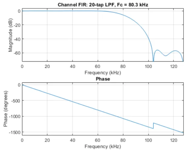
Because the FIR module is reused multiple times, we decided it is important to verify its functionality individually before testing it with the rest of the pipeline. We performed verification on the channel low-pass FIR, since this is the first DSP block that operates directly on the raw complex USRP input. We wrote a MATLAB script channel\_verification() to generate the correct reference behavior of the channel filter, and wrote a testbench that reads the same input file and produces directly comparable output text files. To allow bit-true representation of provided C software in MATLAB, we used MATLAB’s Fixed-Point Designer Toolbox. This allows us to completely replicate the C software’s behavior, while providing us with accesss to MATLAB’s visual interface for plotting.

The script first reads srp.txt which stores the received baseband stream as one hexadecimal byte per line. Since each complex sample is stored in little-endian form, the bytes are ordered \textbf{I Low Byte, I High Byte, Q Low Byte, and Q High Byte}. These four bytes are reconstructed into signed 16-bit I and Q samples. After reconstructing the input, MATLAB designs the channel filter as a 20-tap low-pass filter with a $f_c = 80.3$kHz at a sample rate of $256$ kS/s.

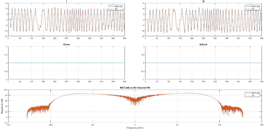
The coefficients are exported to a memory initialization file, channel\_lpf\_20tap.mem, which is used in the RTL simulation. The same fixed-point FIR function is applied separately to I and Q signals, producing matlab\_channel\_i.txt and matlab\_channel\_q.txt outputs. If the RTL-generated outputs are present, the MATLAB scripts reads sv\_channel\_i.txt and sv\_channel\_q.txt and does a sample by sample comparison.

On the RTL side, we performed verification using the modules channel\_fir\_tb.sv and channel\_fir\_top.sv. The top-level wrapper instantiates two copies of the fir.sv module (for the I/Q channels). Both instances use the same coefficient memory file channel\_lpf\_20tap.mem. The testbench reads the usrp.txt file into a byte array, checks that the total number of bytes is a multiple of $4$, and then reconstructs each sample by concatenating the appropriate I and Q bytes. The testbench streams each I/Q pair into channel\_fir\_top.sv using the input valid/ready handshake. The outputs are written to sv\_channel\_i.txt and sv\_channel\_q.txt. This verification proved the RTL outputs are bit-true to the C/MATLAB software.

Demodulation

The demodulation module was the hardest signal processing block to implement in the system. It implements a quadrature FM discriminator that converts complex I/Q samples into a real-valued signal proportional to the instantaneous frequency. Rather than computing phase directly using trigonometric functions, the design uses a cross-product formulation based on consecutive samples. The numerator is computed as $I[n]\cdot Q[n-1] - Q[n] \cdot I[n-1]$, which captures the rotational change of the signal in the complex plane. The denominator is computed as $I[n]^2 +Q[n]^2$, providing amplitude normalization. These operations are implemented using multipliers and adders, with intermediate registers used to store previous samples.

A key design decision in this module is the use of a sequential divider to compute the final ratio. The divider is implemented as a restoring division algorithm that produces one bit of the quotient per clock cycle. This avoids the large combinational logic required for a fully parallel divider and ensures the design remains synthesizable. The tradeoff is increased latency, but this is mitigated by placing FIFOs around the demodulation block so that upstream and downstream modules are not stalled. Careful bit-width selection is required in this module to prevent overflow in the numerator and denominator. This also maintains the correct precision for the output!

Multiplier Block

Our decoder requires a sample-by-sample multiplication at two points in the signal chain. The first is when the extracted stereo pilot tone is squared in order to geneate a component at twice the pilot frequency, which is used as a 38 kHz reference. The second is when this recovered carrier is multiplied by the filtered L-R branch to shift the stereo difference back to baseband. Since both operations are mathematically identical, we decided to make a single reusable fixed-point multiplication block.

The multiplier computes a scaled product of two signed fixed-point input signals. If the two inputs are denoted $a[n]$ and $b[n]$, the output is

where $\text{fix}()$ is truncation towards zero. An direct bitshift scaling of negative numbers results in a floor division, which can result in a systematic error throughout the pipeline. Thus, to replicate the truncation towards zero in hardware, we can add a bias for negative values, like

After scaling, the result is clamped to the representable 32 bit output range:

This saturated value is then registered on the next clock edge. This block is also bit-true to the C/MATLAB software outputs.

Verification

The verification strategy for this project followed two complementary approaches: directed testbenches using C/MATLAB-generated software outputs, and a UVM-based environment for full system validation.

For each major DSP block, including FIR filters, demodulation, and multiplier stages, a corresponding MATLAB script was developed to replicate the exact fixed-point behavior of the reference C implementation. These scripts generated golden output files for each stage of the pipeline, allowing direct comparison against RTL simulation results. The testbenches read input stimulus from text files, streamed data into the DUT using valid-ready handshaking, and wrote outputs to files for comparison.

This approach allowed each module to be verified in isolation before integration. Because the golden outputs were generated from a bit-accurate software model, mismatches could be detected at the sample level, making debugging straightforward. This was especially important for fixed-point arithmetic, where small differences in rounding or scaling can propagate through the system. This was also helpful because test-vectors could be easily generated from MATLAB without changing the testbench structure.

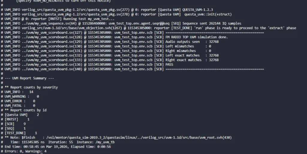
The UVM environment was designed to verify the full fm_radio pipeline under realistic streaming conditions. The environment follows a standard agent-based architecture, consisting of a driver, monitor, sequencer, and scoreboard connected through transaction-level communication. Input stimulus is generated as transactions representing I/Q samples and is driven into the DUT through a virtual interface. The driver converts these transactions into cycle-accurate signals.

The monitor observes the DUT interface and reconstructs output transactions from the streamed data. These transactions are then passed to the scoreboard, which compares them against expected results. The scoreboard uses reference data derived from the same MATLAB/C model used in the directed testbenches, ensuring consistency across both verification approaches. By performing comparisons at the transaction level rather than directly on signals, the UVM environment abstracts away timing differences and focuses on functional correctness.

Sequences are used to control stimulus generation and allow different test scenarios to be exercised without modifying the underlying environment. This enables flexible testing of various input conditions, including continuous streaming, burst traffic, and backpressure scenarios. The configuration object allows parameters such as input file selection and simulation settings to be modified without changing the testbench code. We achieved a complete bit-true comparision to the left_audio.txt and right_audio.txt.

Synthesis

We synthesized our RTL on an Intel Cyclone V.

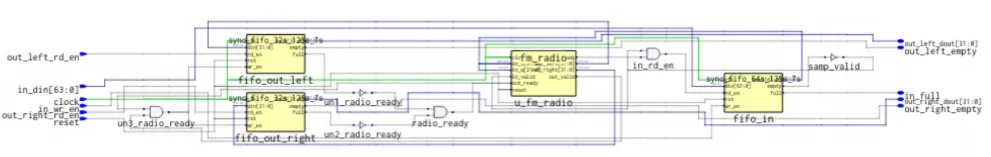
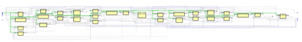
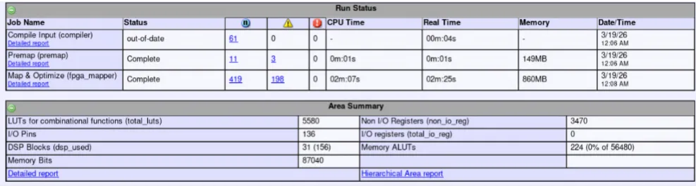
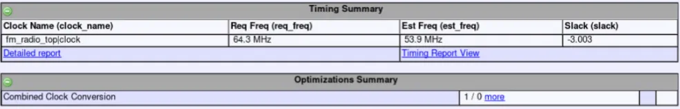
Worst path is from u\_fm\_radio.u\_bp\_p\_ot.u\_fir.x\_reg\_CF4\_0[1]/q\ to u\_fm\_radio.u\_bp\_pilot.u\_fir.out\_data\_reg[0]/sclr, resulting in max freq of about 63.5 MHz. The RTL schematic looks correct because it reflects our intended structural hieararchy. Two input FIFOs feed the buffered sample I and Q sample streams into the \texttt{fm_radio} block, and inside the block we instantiate teh processing pipeline elements such as the FIR filters, demodulation logic, IIR filtering, gain stages, add/sub reconstruction, and external internal FIFOs. The diagram shows the correct data flow with register boundaries and no disconnected modules, which confirms that synthesis recognized our module instantiations correctly and wired correctly. From a connectivity standpoint, it looks correct!

However, negative slack means a data path is arriving too late for the required clock period. 3 ns is pretty significant, and the possible options we have to fix it is to either reduce the clock frequency, add registers (pipelining) in long combinational paths, and improve constraints. So while the RTL ‘works’ conceptually, there is still work to be done until the design is ready to be programmed into a physical FPGA.