Open Table of Contents

Simulation

Simulation Output

You may need to click play a couple times (or pause then play) to get the simulation started

Introduction

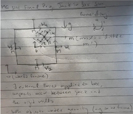
For my final project, I simulated the dynamics of a 2 dimensional jack-in-the-box system. There are external forces applied on the box and impacts aoccur between the rigid bodies of the jack’s endpoints and the box’s walls.

Two external forces are applied to the box the first is an equal and opposite force to gravity (to ensure the box stays at the same position and doesn’t move vertically), and the second is a torque to rotate the box. The torque is a function of frequency that changes over with time (like a weird chirp), but the box will continue to rotate in the same direcition. The rigid bodies are also subject to gravity, which is directed in the -y direction of the world frame. In the following sections, I’ll explain the equation setups, some derivations, and simulation outputs.

Imports

Throughout the class, we utilized sympy, a symbolic math library, for deriving the equations of motion (EOM).

import numpy as np
import sympy as sym
from sympy.abc import t
from sympy import sin, cos, symbols, Function, Inverse, Eq, Matrix, Rational, simplify, lambdify, solve
from math import pi
import matplotlib.pyplot as plt

Santa’s Little Helper Functions

def mat_inverse(g):
    ''' Inverse operations
    '''
    R = Matrix([[g[0,0], g[0,1], g[0,2]],
                [g[1,0], g[1,1], g[1,2]],
                [g[2,0], g[2,1], g[2,2]]])
    R_inv = R.T
    p = Matrix([g[0,3], g[1,3], g[2,3]])
    p_inv = -R_inv * p
    g_inv = Matrix([[R_inv[0,0], R_inv[0,1], R_inv[0,2], p_inv[0]],
                      [R_inv[1,0], R_inv[1,1], R_inv[1,2], p_inv[1]],
                      [R_inv[2,0], R_inv[2,1], R_inv[2,2], p_inv[2]],
                      [         0,          0,         0,        1]])
    return g_inv
def unhat(g):
    ''' Unhatting operations...
    '''
    V = Matrix([0, 0, 0, 0, 0, 0])
    V[0, 0] = g[0, 3]
    V[1, 0] = g[1, 3]
    V[2, 0] = g[2, 3]
    V[3, 0] = g[2, 1]
    V[4, 0] = g[0, 2]
    V[5, 0] = g[1, 0]

    return V
def get_se3_np(x, y, theta):
    """
    Given a rotation about theta (CCW), and translation p = [x y]T, finds se3 matrix
    """
    return np.array([[np.cos(theta), -np.sin(theta), 0, x],
                     [np.sin(theta),  np.cos(theta), 0, y],
                     [            0,              0, 1, 0],
                     [            0,              0, 0, 1]])
def integrate(f, xt, dt, time):
    """
    This function takes in an initial condition x(t) and a timestep dt,
    as well as a dynamical system f(x) that outputs a vector of the
    same dimension as x(t). It outputs a vector x(t+dt) at the future
    time step.

    Parameters
    ============
    dyn: Python function
        derivate of the system at a given step x(t),
        it can considered as \dot{x}(t) = func(x(t))
    x0: NumPy array
        current step x(t)
    dt:
        step size for integration
    time:
        step time

    Return
    ============
    new_x:
        value of x(t+dt) integrated from x(t)
    """
    k1 = dt * f(xt, time)
    k2 = dt * f(xt+k1/2., time)
    k3 = dt * f(xt+k2/2., time)
    k4 = dt * f(xt+k3, time)
    new_xt = xt + (1/6.) * (k1+2.0*k2+2.0*k3+k4)

    return new_xt
def simulate_impact(f, x0, tspan, dt, integrate):
    """
    This function takes in an initial condition x0, a timestep dt,
    a time span tspan consisting of a list [min_time, max_time],
    as well as a dynamical system f(x) that outputs a vector of the
    same dimension as x0. It outputs a full trajectory simulated
    over the time span of dimensions (xvec_size, time_vec_size).

    Parameters
    ============
    f: Python function
        derivate of the system at a given step x(t),
        it can considered as \dot{x}(t) = func(x(t))
    x0: NumPy array
        initial conditions
    tspan: Python list
        tspan = [min_time, max_time], it defines the start and end
        time of simulation
    dt:
        time step for numerical integration
    integrate: Python function
        numerical integration method used in this simulation

    Return
    ============
    x_traj:
        simulated trajectory of x(t) from t=0 to tf
    """
    N = int((max(tspan)-min(tspan))/dt)
    x = np.copy(x0)
    tvec = np.linspace(min(tspan),max(tspan), N)
    xtraj = np.zeros((len(x0), N))
    time = 0
    for i in range(N):
        time = time + dt
        (impact, impact_num) = impact_condition(x, phi_func, 1e-1)
        if impact is True:
            x = impact_update(x, impact_eqns_list[impact_num], dum_list)
            xtraj[:, i]=integrate(f, x, dt, time)
        else:
            xtraj[:, i]=integrate(f, x, dt, time)
        x = np.copy(xtraj[:,i])
    return xtraj

mat(g)

Inverts a 4×4 homogeneous transformation matrix $g \in SE(3)$ .

If:

g = \begin{bmatrix} R & p \\ 0 & 1 \end{bmatrix}

Then:

g^{-1} = \begin{bmatrix} R^T & -R^T p \\ 0 & 1 \end{bmatrix}

Used to reverse coordinate transforms.

unhat(g)

Extracts a 6×1 twist vector $\xi$ from a 4×4 matrix in $\mathfrak{se}(3)$ .

Returns:

\xi = \begin{bmatrix} v \\ \omega \end{bmatrix}

Where $v$ is the translational part and $\omega$ comes from the skew-symmetric rotational component of $g$ .

get_se3_np(x, y, \theta)

Returns a 4×4 transformation matrix in $SE(3)$ for a planar rigid body located at $(x, y)$ with orientation $\theta$ (CCW):

g = \begin{bmatrix} \cos \theta & -\sin \theta & 0 & x \\ \sin \theta & \cos \theta & 0 & y \\ 0 & 0 & 1 & 0 \\ 0 & 0 & 0 & 1 \end{bmatrix}

Assumes planar motion (no $z$ translation or tilt).

integrate(f, x_t, dt, time)

Fourth-order Runge-Kutta integrator to advance $x(t)$ forward by $\Delta t$ :

\begin{aligned} k_1 &= f(x_t, t) \cdot dt \\ k_2 &= f(x_t + \frac{k_1}{2}, t) \cdot dt \\ k_3 &= f(x_t + \frac{k_2}{2}, t) \cdot dt \\ k_4 &= f(x_t + k_3, t) \cdot dt \\ x_{t+dt} &= x_t + \frac{1}{6}(k_1 + 2k_2 + 2k_3 + k_4) \end{aligned}

Used for time-stepping the continuous dynamics.

simulateimpact(f, x_0, $t{\text{span}}$ , dt, $\text{integrate}$ )

Simulates system dynamics over time, accounting for impacts with discrete changes in velocity or constraint enforcement.

At each timestep:

Check for impact with impact_condition(...)
If an impact occurs:
- Update the state with impact_update(...)
Otherwise integrate normally

Returns full trajectory matrix:

Shape: $(\text{state\_dim} \times \text{num\_timesteps})$

Dependencies (not defined yet):

impact_condition(x, φ, ε): Returns whether collision occurred
impact_update(x, eqns, dummies): Applies post-impact velocity changes
phi_func: Constraint/impact condition function
impact_eqns_list, dum_list: Precomputed symbolic expressions for impacts

System Parameters, Transformations, and Lagrangian Derivation

schematic

Here, I define system geometry, mass properties, external forces, and use sympy to solve the Euler-Lagrange equations of motion.

  # Box parameters:
l_box, M_box = 6, 100
j_box = 4*M_box*l_box**2
# parameters of jack:
l_jack, m_jack = 1, 1
j_jack = 4*m_jack*l_jack**2
g = 9.81
# Define box and jack's position and orientatino:
x_box = Function(r'x_box')(t)
y_box = Function(r'y_box')(t)
theta_box = Function(r'\theta_box')(t)
x_jack = Function(r'x_jack')(t)
y_jack = Function(r'y_jack')(t)
theta_jack = Function(r'\theta_jack')(t)

# external forces on box (torque + vertical force acting on center of box):
deltaT = 1
f_0 = 1
f_f = 5
c = (f_f - f_0)/deltaT
# theta_d_box = sin(2*pi/5*(0.5*c*t**2+f_0*t))
# theta_d_box = sin((2*pi/5)*t)

# New chirp signal:
A = 3  # Adjust amplitude as needed
f0 = 0.5  # Initial frequency
k = 0.9  # Chirp rate
theta_d_box = A * sin(2 * pi * (f0 * t + 0.5 * k * t**2))

k = 30000
F_y_box = 4*M_box*g
F_theta_box = k*(theta_d_box)
F = Matrix([0, F_y_box, F_theta_box, 0, 0, 0])

# Config Vars of system:
q = Matrix([x_box, y_box, theta_box, x_jack, y_jack, theta_jack])
qdot = q.diff(t)
qddot = qdot.diff(t)

# Homogeonous reps of the rigid bodies:
g_w_b = Matrix([[cos(theta_box), -sin(theta_box), 0, x_box], [sin(theta_box), cos(theta_box), 0, y_box], [0, 0, 1, 0], [0, 0, 0, 1]])
g_b_b1 = Matrix([[1, 0, 0, l_box], [0, 1, 0, l_box], [0, 0, 1, 0], [0, 0, 0, 1]])
g_b_b2 = Matrix([[1, 0, 0, 0], [0, 1, 0, -l_box], [0, 0, 1, 0], [0, 0, 0, 1]])
g_b_b3 = Matrix([[1, 0, 0, -l_box], [0, 1, 0, 0], [0, 0, 1, 0], [0, 0, 0, 1]])
g_b_b4 = Matrix([[1, 0, 0, 0], [0, 1, 0, l_box], [0, 0, 1, 0], [0, 0, 0, 1]])
g_w_j = Matrix([[cos(theta_jack), -sin(theta_jack), 0, x_jack], [sin(theta_jack), cos(theta_jack), 0, y_jack], [0, 0, 1, 0], [0, 0, 0, 1]])
g_j_j1 = Matrix([[1, 0, 0, l_jack], [0, 1, 0, 0], [0, 0, 1, 0], [0, 0, 0, 1]])
g_j_j2 = Matrix([[1, 0, 0, 0], [0, 1, 0, -l_jack], [0, 0, 1, 0], [0, 0, 0, 1]])
g_j_j3 = Matrix([[1, 0, 0, -l_jack], [0, 1, 0, 0], [0, 0, 1, 0], [0, 0, 0, 1]])
g_j_j4 = Matrix([[1, 0, 0, 0], [0, 1, 0, l_jack], [0, 0, 1, 0], [0, 0, 0, 1]])

g_w_b1 = g_w_b * g_b_b1
g_w_b2 = g_w_b * g_b_b2
g_w_b3 = g_w_b * g_b_b3
g_w_b4 = g_w_b * g_b_b4

g_w_j1 = g_w_j * g_j_j1
g_w_j2 = g_w_j * g_j_j2
g_w_j3 = g_w_j * g_j_j3
g_w_j4 = g_w_j * g_j_j4

g_b1_j1 = mat_inverse(g_w_b1) * g_w_j1
g_b1_j2 = mat_inverse(g_w_b1) * g_w_j2
g_b1_j3 = mat_inverse(g_w_b1) * g_w_j3
g_b1_j4 = mat_inverse(g_w_b1) * g_w_j4

g_b2_j1 = mat_inverse(g_w_b2) * g_w_j1
g_b2_j2 = mat_inverse(g_w_b2) * g_w_j2
g_b2_j3 = mat_inverse(g_w_b2) * g_w_j3
g_b2_j4 = mat_inverse(g_w_b2) * g_w_j4

g_b3_j1 = mat_inverse(g_w_b3) * g_w_j1
g_b3_j2 = mat_inverse(g_w_b3) * g_w_j2
g_b3_j3 = mat_inverse(g_w_b3) * g_w_j3
g_b3_j4 = mat_inverse(g_w_b3) * g_w_j4

g_b4_j1 = mat_inverse(g_w_b4) * g_w_j1
g_b4_j2 = mat_inverse(g_w_b4) * g_w_j2
g_b4_j3 = mat_inverse(g_w_b4) * g_w_j3
g_b4_j4 = mat_inverse(g_w_b4) * g_w_j4

#Rigid body velocity of box and jack:
V_box = unhat(mat_inverse(g_w_b) * g_w_b.diff(t))
V_jack = unhat(mat_inverse(g_w_j) * g_w_j.diff(t))

# Inertia Matrices of jack and box:
I_box = Matrix([[4*M_box, 0, 0, 0, 0, 0], [0, 4*M_box, 0, 0, 0, 0], [0 ,0 ,4*M_box ,0 ,0 ,0], [0, 0, 0, 0, 0, 0], [0, 0, 0, 0, 0, 0], [0, 0, 0, 0, 0, j_box]])
I_jack = Matrix([[4*m_jack, 0, 0, 0, 0, 0], [0, 4*m_jack, 0, 0, 0, 0], [0, 0, 4*m_jack, 0, 0, 0], [0, 0, 0, 0, 0, 0], [0, 0, 0 ,0, 0, 0], [0, 0, 0, 0, 0, j_jack]])

# System Lagrangian Calculation:
KE = simplify(0.5*(V_box.T)*I_box*V_box + 0.5*(V_jack.T)*I_jack*V_jack)[0]
PE = simplify(g*(4*M_box*y_box + 4*m_jack*y_jack))
L = simplify(KE - PE)

# Compute EL Equations:
dL_dq = simplify(Matrix([L]).jacobian(q).T)
dL_dqdot = simplify(Matrix([L]).jacobian(qdot).T)
ddL_dqdot_dt = simplify(dL_dqdot.diff(t))

lhs = simplify(ddL_dqdot_dt - dL_dq)
rhs = simplify(F)
EL_Eqs = simplify(Eq(lhs, rhs))
display(EL_Eqs)

# Solving EL Equations:
EL_solns = solve(EL_Eqs, qddot, dict=True)

Parameters

Box:
- Side length $l_{\text{box}} = 6$
- Mass $M_{\text{box}} = 100$
- Moment of inertia:
  $j*{\text{box}} = 4 M*{\text{box}} l\_{\text{box}}^2$
Jack:
- Length $l_{\text{jack}} = 1$
- Mass $m_{\text{jack}} = 1$
- Moment of inertia:
  $j*{\text{jack}} = 4 m*{\text{jack}} l\_{\text{jack}}^2$
Gravity: $g = 9.81$

Generalized Coordinates

The positions and orientations of the box and jack are defined as time-varying symbolic functions:

$x_{\text{box}}(t)$ , $y_{\text{box}}(t)$ , $\theta_{\text{box}}(t)$
$x_{\text{jack}}(t)$ , $y_{\text{jack}}(t)$ , $\theta_{\text{jack}}(t)$

These form the generalized coordinate vector:

q = \begin{bmatrix} x_{\text{box}} \\ y_{\text{box}} \\ \theta_{\text{box}} \\ x_{\text{jack}} \\ y_{\text{jack}} \\ \theta_{\text{jack}} \end{bmatrix}

External Forces

A vertical force $F_y$ and a torque $F_\theta$ are applied to the box.

Vertical force: $F*y = 4 M*{\text{box}} g$
Torque input:
A chirp signal defines the desired rotation:
$\theta_d(t) = A \sin \left( 2\pi\left( f_0 t + \frac{1}{2} k t^2 \right) \right)$
Then the torque is:
$F_\theta = k \cdot \theta_d(t)$

The force vector becomes:

F = \begin{bmatrix} 0 \\ F_y \\ F_\theta \\ 0 \\ 0 \\ 0 \end{bmatrix}

Rigid Body Transforms

g_w_b and g_w_j define the homogeneous transforms from the world to the box and jack respectively.
g_b_b1 to g_b_b4, and g_j_j1 to g_j_j4 represent local frames at box/jack corners.
Transforms to world frame: $g_{w}^{b_i} = g_{w}^{b} \cdot g_{b}^{b_i}, \quad g_{w}^{j_i} = g_{w}^{j} \cdot g_{j}^{j_i}$
Relative transforms (used for constraints or geometric relationships): $g_{b_i}^{j_j} = (g_w^{b_i})^{-1} \cdot g_w^{j_j}$

Rigid Body Velocities

Using the matrix logarithmic map and the time derivative of transforms:

V_{\text{box}} = \text{unhat}\left( g_{w}^{b^{-1}} \cdot \frac{d}{dt} g_{w}^{b} \right), \quad V_{\text{jack}} = \text{unhat}\left( g_{w}^{j^{-1}} \cdot \frac{d}{dt} g_{w}^{j} \right)

Inertia Matrices

Mass and rotational inertia expressed as 6D spatial inertia matrices:

I = \begin{bmatrix} m I_{3 \times 3} & 0 \\ 0 & J \end{bmatrix}

For the box: $I*{\text{box}} = \text{diag}(4 M*{\text{box}}, 4 M*{\text{box}}, 4 M*{\text{box}}, 0, 0, j\_{\text{box}})$
For the jack: $I*{\text{jack}} = \text{diag}(4 m*{\text{jack}}, 4 m*{\text{jack}}, 4 m*{\text{jack}}, 0, 0, j\_{\text{jack}})$

Lagrangian Formulation

Kinetic Energy:
$KE = \frac{1}{2} V_{\text{box}}^\top I_{\text{box}} V_{\text{box}} + \frac{1}{2} V_{\text{jack}}^\top I_{\text{jack}} V_{\text{jack}}$
Potential Energy:
$PE = g (4 M_{\text{box}} y_{\text{box}} + 4 m_{\text{jack}} y_{\text{jack}})$
Lagrangian:
$\mathcal{L} = KE - PE$

Solving EL Equations

We compute:

$\frac{\partial \mathcal{L}}{\partial q}$
$\frac{d}{dt} \left( \frac{\partial \mathcal{L}}{\partial \dot{q}} \right)$

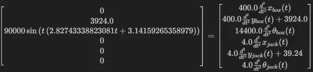
The final equations of motion are:

\frac{d}{dt} \left( \frac{\partial \mathcal{L}}{\partial \dot{q}} \right) - \frac{\partial \mathcal{L}}{\partial q} = F

This gives a system of 6 second-order differential equations in $q(t)$ .

The solve line yields the following expressions for the generalized accelerations $\ddot{q}$ .

solved EOMs

Numerical Integration of System Dynamics

This section converts the symbolic Euler-Lagrange solutions into numerical functions using lambdify, and defines a simulation-ready dynamics function to be used in numerical integrators (e.g. odeint or solve_ivp).

#Lambdifying
x_box_ddot_func = lambdify([q[0], q[1], q[2], q[3], q[4], q[5], qdot[0], qdot[1], qdot[2], qdot[3], qdot[4], qdot[5], t], EL_solns[0][qddot[0]])
y_box_ddot_func = lambdify([q[0], q[1], q[2], q[3], q[4], q[5], qdot[0], qdot[1], qdot[2], qdot[3], qdot[4], qdot[5], t], EL_solns[0][qddot[1]])
theta_box_ddot_func = lambdify([q[0], q[1], q[2], q[3], q[4], q[5], qdot[0], qdot[1], qdot[2], qdot[3], qdot[4], qdot[5], t], EL_solns[0][qddot[2]])
x_jack_ddot_func = lambdify([q[0], q[1], q[2], q[3], q[4], q[5], qdot[0], qdot[1], qdot[2], qdot[3], qdot[4], qdot[5], t], EL_solns[0][qddot[3]])
y_jack_ddot_func = lambdify([q[0], q[1], q[2], q[3], q[4], q[5], qdot[0], qdot[1], qdot[2], qdot[3], qdot[4], qdot[5], t], EL_solns[0][qddot[4]])
theta_jack_ddot_func = lambdify([q[0], q[1], q[2], q[3], q[4], q[5], qdot[0], qdot[1], qdot[2], qdot[3], qdot[4], qdot[5], t], EL_solns[0][qddot[5]])

def dynamics(s, t):
    sdot = np.array([
        s[6],
        s[7],
        s[8],
        s[9],
        s[10],
        s[11],
        x_box_ddot_func(*s, t),
        y_box_ddot_func(*s, t),
        theta_box_ddot_func(*s, t),
        x_jack_ddot_func(*s, t),
        y_jack_ddot_func(*s, t),
        theta_jack_ddot_func(*s, t)
    ])
    return sdot


# Acceleration Matrix
qddot_Matrix = Matrix([qdot[0], EL_solns[0][qddot[0]],
                       qdot[1], EL_solns[0][qddot[1]],
                       qdot[2], EL_solns[0][qddot[2]],
                       qdot[3], EL_solns[0][qddot[3]],
                       qdot[4], EL_solns[0][qddot[4]],
                       qdot[5], EL_solns[0][qddot[5]]])

# Dummy syms:
x_b_l, y_b_l, theta_b_l, x_j_l, y_j_l, theta_j_l, x_b_ldot, y_b_ldot, theta_b_ldot, x_j_ldot, y_j_ldot, theta_j_ldot = symbols('x_box_l, y_box_l, theta_box_l, x_jack_l, y_jack_l, theta_jack_l, x_box_ldot, y_box_ldot, theta_box_ldot, x_jack_ldot, y_jack_ldot, theta_jack_ldot')

dummy_dict = {q[0]:x_b_l, q[1]:y_b_l, q[2]:theta_b_l,
              q[3]:x_j_l, q[4]:y_j_l, q[5]:theta_j_l,
              qdot[0]:x_b_ldot, qdot[1]:y_b_ldot, qdot[2]:theta_b_ldot,
              qdot[3]:x_j_ldot, qdot[4]:y_j_ldot, qdot[5]:theta_j_ldot}
qddot_d = qddot_Matrix.subs(dummy_dict)
qddot_lambdify = lambdify([x_b_l, x_b_ldot ,y_b_l, y_b_ldot, theta_b_l, theta_b_ldot,
                           x_j_l, x_j_ldot ,y_j_l, y_j_ldot, theta_j_l, theta_j_ldot, t], qddot_d)

Lambdified Acceleration Functions

Each component of the acceleration vector $\ddot{q}$ is turned into a callable Python function. The inputs are:

The full state: $q$ and $\dot{q}$ (i.e., 12 state variables)
Time $t$

Example:

x_box_ddot_func = lambdify([...], EL_solns[0][qddot[0]])

This allows numerical evaluation of:

\ddot{x}_{\text{box}} = f(q, \dot{q}, t)

Dynamics Function

A full dynamics function is defined to return $\dot{s}$ (derivative of the state vector):

def dynamics(s, t):
    sdot = np.array([...])
    return sdot

Where:

$s = [q_1, q_2, ..., q_6, \dot{q}_1, \dot{q}_2, ..., \dot{q}_6]$
$s_{\text{dot}} = [\dot{q}_1, ..., \dot{q}_6, \ddot{q}_1, ..., \ddot{q}_6]$

This function is suitable for numerical integration with methods like:

odeint(dynamics, s0, t_array)

Acceleration Matrix

We also define a symbolic matrix of interleaved velocities and accelerations:

\begin{bmatrix} \dot{q}_1 \\ \ddot{q}_1 \\ \dot{q}_2 \\ \ddot{q}_2 \\ \vdots \\ \dot{q}_6 \\ \ddot{q}_6 \\ \end{bmatrix}

This is helpful for vectorizing evaluations and computing Jacobians later.

Dummy Symbol Substitution

To allow symbolic manipulation independent of the original symbolic variables, dummy symbols are created:

x_b_l, y_b_l, theta_b_l, ...

A substitution dictionary maps the symbolic variables $q_i$ and $\dot{q}_i$ to these dummy symbols:

dummy_dict = { q[0]: x_b_l, qdot[0]: x_b_ldot, ... }

This produces qddot_d, a dummy-labeled version of the acceleration matrix, and then:

qddot_lambdify = lambdify([...], qddot_d)

Which allows evaluation of all state derivatives from a new state vector input format:

[x_{\text{box}}, \dot{x}_{\text{box}}, y_{\text{box}}, \dot{y}_{\text{box}}, \theta_{\text{box}}, \dot{\theta}_{\text{box}}, \ldots]

Impact Modeling with Constraints and Energy Conservation

This section introduces impact constraints for when the jack collides with the interior walls of the box. It formulates the constraint conditions symbolically, computes their Jacobians, and finally sets up equations to enforce conservation of momentum and energy consistency during impacts.

r_jack_hat = Matrix([x_jack, y_jack, theta_jack, 1])

# Impact constraint for wall 1:
phi_b1_j1 = (g_b1_j1[3]).subs(dummy_dict)
phi_b1_j2 = (g_b1_j2[3]).subs(dummy_dict)
phi_b1_j3 = (g_b1_j3[3]).subs(dummy_dict)
phi_b1_j4 = (g_b1_j4[3]).subs(dummy_dict)

# Impact constraint for wall 2:
phi_b2_j1 = (g_b2_j1[7]).subs(dummy_dict)
phi_b2_j2 = (g_b2_j2[7]).subs(dummy_dict)
phi_b2_j3 = (g_b2_j3[7]).subs(dummy_dict)
phi_b2_j4 = (g_b2_j4[7]).subs(dummy_dict)

# Impact constraint for wall 3:
phi_b3_j1 = (g_b3_j1[3]).subs(dummy_dict)
phi_b3_j2 = (g_b3_j2[3]).subs(dummy_dict)
phi_b3_j3 = (g_b3_j3[3]).subs(dummy_dict)
phi_b3_j4 = (g_b3_j4[3]).subs(dummy_dict)

# Impact constraint for wall 4:
phi_b4_j1 = (g_b4_j1[7]).subs(dummy_dict)
phi_b4_j2 = (g_b4_j2[7]).subs(dummy_dict)
phi_b4_j3 = (g_b4_j3[7]).subs(dummy_dict)
phi_b4_j4 = (g_b4_j4[7]).subs(dummy_dict)

# System Impact constraint:
phi_dum = simplify(Matrix([[phi_b1_j1], [phi_b1_j2], [phi_b1_j3], [phi_b1_j4],  # all jack frames in the box1 frame
                           [phi_b2_j1], [phi_b2_j2], [phi_b2_j3], [phi_b2_j4],  # all jack frames in the box2 frame
                           [phi_b3_j1], [phi_b3_j2], [phi_b3_j3], [phi_b3_j4],  # all jack frames in the box3 frame
                           [phi_b4_j1], [phi_b4_j2], [phi_b4_j3], [phi_b4_j4]])) # all jack frames in the box4 frame

# Hamiltonain Calculation:
H = simplify((dL_dqdot.T * qdot)[0] - L)

# Evaluate expressions:
H_dum = H.subs(dummy_dict)
dL_dqdot_dum = dL_dqdot.subs(dummy_dict)
dPhidq_dum = phi_dum.jacobian([x_b_l, y_b_l, theta_b_l, x_j_l, y_j_l, theta_j_l])

# tau+ dummy sym:
lamb = symbols(r'lambda')
x_b_dot_Plus, y_b_dot_Plus, theta_b_dot_Plus, x_j_dot_Plus, y_j_dot_Plus, theta_j_dot_Plus = symbols(r'x_box_dot_+, y_box_dot_+, theta_box_dot_+, x_jack_dot_+, y_jack_dot_+, theta_jack_dot_+')

impact_dict = {x_b_ldot:x_b_dot_Plus, y_b_ldot:y_b_dot_Plus, theta_b_ldot:theta_b_dot_Plus,
               x_j_ldot:x_j_dot_Plus, y_j_ldot:y_j_dot_Plus, theta_j_ldot:theta_j_dot_Plus}

# Eval at tau+:
dL_dqdot_dumPlus = simplify(dL_dqdot_dum.subs(impact_dict))
dPhidq_dumPlus = simplify(dPhidq_dum.subs(impact_dict))
H_dumPlus = simplify(H_dum.subs(impact_dict))

impact_eqns_list = []

# Constrained impact equations
lhs = Matrix([dL_dqdot_dumPlus[0] - dL_dqdot_dum[0],
              dL_dqdot_dumPlus[1] - dL_dqdot_dum[1],
              dL_dqdot_dumPlus[2] - dL_dqdot_dum[2],
              dL_dqdot_dumPlus[3] - dL_dqdot_dum[3],
              dL_dqdot_dumPlus[4] - dL_dqdot_dum[4],
              dL_dqdot_dumPlus[5] - dL_dqdot_dum[5],
              H_dumPlus - H_dum])

for i in range(phi_dum.shape[0]):
    rhs = Matrix([lamb*dPhidq_dum[i,0],
                  lamb*dPhidq_dum[i,1],
                  lamb*dPhidq_dum[i,2],
                  lamb*dPhidq_dum[i,3],
                  lamb*dPhidq_dum[i,4],
                  lamb*dPhidq_dum[i,5],
                  0])
    impact_eqns_list.append(simplify(Eq(lhs, rhs)))

Jack Pose Vector

The jack configuration is packaged into a homogeneous vector:

r_jack_hat = Matrix([x_jack, y_jack, theta_jack, 1])

This allows multiplication with homogeneous transformation matrices like $g_{b}^{j}$ to get spatial relationships.

Impact Constraints

Each box wall (1 through 4) is tested for collisions against each jack endpoint (1 through 4). For example:

phi_b1_j1 = g_b1_j1[3] extracts the x-position component of jack frame 1 in box frame 1.
phi_b2_j1 = g_b2_j1[7] extracts the y-position for checking vertical constraints.

These constraint values $\phi$ are symbolic expressions which should evaluate to zero when impact occurs.

The full list of constraints is stacked into a column vector:

\phi(q, \dot{q}) = \begin{bmatrix} \phi_{b1,j1} \\ \phi_{b1,j2} \\ \vdots \\ \phi_{b4,j4} \end{bmatrix}

Hamiltonian

To handle impacts, we define the system Hamiltonian:

H = \dot{q}^T \frac{\partial \mathcal{L}}{\partial \dot{q}} - \mathcal{L}

We then substitute dummy symbolic variables (like x_b_ldot) for generalization:

H_dum = H.subs(dummy_dict)

Jacobian of Constraints

We compute:

\frac{\partial \phi}{\partial q}

This Jacobian tells us how each constraint varies with generalized coordinates. It’s essential for computing reaction impulses during impacts.

Impact Equations at τ⁺

We evaluate generalized momenta just after impact $\tau^+$ :

Replace all $\dot{q}_i$ $\overset{q}{˙}_{i}$ with their post-impact versions, e.g.:
- $\dot{x}_{\text{box}} \mapsto \dot{x}_{\text{box}}^+$
Define impact equations as:
- Difference in momenta before and after = constraint force term: $\frac{\partial \mathcal{L}}{\partial \dot{q}}(\tau^+) - \frac{\partial \mathcal{L}}{\partial \dot{q}}(\tau^-) = \lambda \cdot \frac{\partial \phi}{\partial q}$
- Also include conservation of energy: $H(\tau^+) = H(\tau^-)$

The full left-hand side becomes:

lhs = [Δp_1, Δp_2, ..., Δp_6, ΔH]

And the right-hand side:

rhs = λ * ∇φ (for each constraint)

Final Assembly of Equations

Each constraint yields a 7-dimensional vector equation (6 momentum components + 1 Hamiltonian):

Loop over all constraints (16 total):
Plug in corresponding rows of the constraint Jacobian
Build:
```
Eq(lhs, rhs)
```

Stored in:

impact_eqns_list

This results in a list of symbolic equations that govern how the system should behave at collisions — capturing the correct impulses and preserving total energy.

Impact Detection and Handling

This section provides a runtime mechanism to detect and resolve impacts during numerical simulation. It includes:

A function to evaluate whether an impact occurs
A solver to compute the post-impact state
Integration with symbolic expressions derived earlier

phi_func = lambdify([x_b_l, y_b_l, theta_b_l,
                     x_j_l, y_j_l, theta_j_l,
                     x_b_ldot, y_b_ldot, theta_b_ldot,
                     x_j_ldot, y_j_ldot, theta_j_ldot],
                    phi_dum)

def impact_condition(s, phi_func, threshold = 1e-1):
    """ Checks system for impact. If impact (abs(phi_val) < threshold)),
    returns 'True' row in phi where imapcts.
    """
    phi_val = phi_func(*s)
    for i in range(phi_val.shape[0]):
        if (phi_val[i] > -threshold) and (phi_val[i] < threshold):
            return (True, i)
    return (False, None)

dum_list = [x_b_dot_Plus, y_b_dot_Plus, theta_b_dot_Plus,
            x_j_dot_Plus, y_j_dot_Plus, theta_j_dot_Plus]

def impact_update(s, impact_eqns, dum_list):
    """ returns the updated state vars after impact impact
    """
    subs_dict = {x_b_l:s[0], y_b_l:s[1], theta_b_l:s[2],
                 x_j_l:s[3], y_j_l:s[4], theta_j_l:s[5],
                 x_b_ldot:s[6], y_b_ldot:s[7], theta_b_ldot:s[8],
                 x_j_ldot:s[9], y_j_ldot:s[10], theta_j_ldot:s[11]}
    new_impact_eqns = impact_eqns.subs(subs_dict)
    impact_solns = solve(new_impact_eqns, [x_b_dot_Plus, y_b_dot_Plus, theta_b_dot_Plus,
                                           x_j_dot_Plus, y_j_dot_Plus, theta_j_dot_Plus,
                                           lamb], dict=True)
    if len(impact_solns) == 1:
        print("Only one solutions")

    else:
        for sol in impact_solns:
            lamb_sol = sol[lamb]
            if abs(lamb_sol) < 1e-06:
                pass
            else:
                return np.array([
                    s[0], #q will be the same after impact
                    s[1],
                    s[2],
                    s[3],
                    s[4],
                    s[5],
                    float(sym.N(sol[dum_list[0]])), #q_dot will change after impact
                    float(sym.N(sol[dum_list[1]])),
                    float(sym.N(sol[dum_list[2]])),
                    float(sym.N(sol[dum_list[3]])),
                    float(sym.N(sol[dum_list[4]])),
                    float(sym.N(sol[dum_list[5]])),
                ])

Lambdifying the Constraint Function

We define a callable version of the stacked impact constraint vector $\phi$ :

phi_func = lambdify([...], phi_dum)

This takes the current state $s = [q, \dot{q}]$ and evaluates all 16 jack-to-wall constraint conditions.

Impact Detection Function

def impact_condition(s, phi_func, threshold = 1e-1):

This function checks whether any of the $\phi_i$ constraints fall within a narrow range around zero:

-\varepsilon < \phi_i < \varepsilon

This means a jack foot is near a wall. The function returns:

True and the index i of the constraint when an impact is detected
False otherwise

This mechanism allows the simulator to switch modes and apply an impulse update when impact occurs.

Variables for Post-Impact Velocities

We use a list of symbols representing the velocities just after impact:

dum_list = [
  \dot{x}_{\text{box}}^+,
  \dot{y}_{\text{box}}^+,
  \dot{\theta}_{\text{box}}^+,
  \dot{x}_{\text{jack}}^+,
  \dot{y}_{\text{jack}}^+,
  \dot{\theta}_{\text{jack}}^+
]

These are used when solving the symbolic impact equations.

Impact Update Function

def impact_update(s, impact_eqns, dum_list)

This function:

Substitutes current state $q$ , $\dot{q}$ into the symbolic impact equations
Solves for the post-impact velocities and Lagrange multiplier $\lambda$
Returns an updated state vector $s^+$

Steps:

1. Substitution

subs_dict = {q_i: s[i], \dot{q}_i: s[i+6]}

Used to evaluate the symbolic impact equations numerically.

2. Solve

impact_solns = solve(new_impact_eqns, [..., λ], dict=True)

Finds all valid solutions to the momentum + constraint system.

3. Select Valid Solution

We check if the Lagrange multiplier $\lambda$ (contact impulse) is non-zero, indicating a meaningful impact:

if abs(lamb_sol) > 1e-6:
    return updated state

This avoids selecting spurious solutions (e.g., zero-impulse).

Output

If a valid solution is found, the function returns:

s^+ = \begin{bmatrix} q_1 \\ \vdots \\ q_6 \\ \dot{q}_1^+ \\ \vdots \\ \dot{q}_6^+ \end{bmatrix}

Otherwise, the simulation continues using standard dynamics integration.

Simulation

This section simulates the time evolution of the box-jack system over a finite time interval using the dynamics and impact handling previously defined.

# Simulate the motion:
tspan = [0, 10]
dt = 0.01
s0 = np.array([0, 0, 0, 0, 0, 0, 0, 0, 0, 0, 0, 0])

N = int((max(tspan) - min(tspan))/dt)
tvec = np.linspace(min(tspan), max(tspan), N)
traj = simulate_impact(dynamics, s0, tspan, dt, integrate)

plt.figure()
plt.plot(tvec, traj[6], label='x_box_dot')
plt.plot(tvec, traj[7], label='y_box_dot')
plt.plot(tvec, traj[8], label='theta_box_dot')
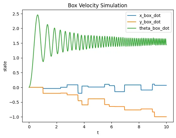
plt.title('Box Velocity Simulation')
plt.xlabel('t')
plt.ylabel('state')
plt.legend(loc="best")
plt.show()

plt.figure()
plt.plot(tvec, traj[9], label='x_jack_dot')
plt.plot(tvec, traj[10], label='y_jack_dot')
plt.plot(tvec, traj[11], label='theta_jack_dot')
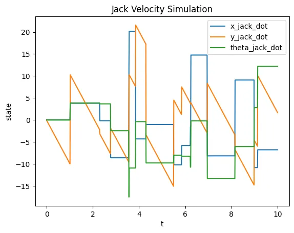
plt.title('Jack Velocity Simulation')
plt.xlabel('t')
plt.ylabel('state')
plt.legend(loc="best")
plt.show()

plt.figure()
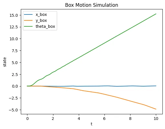
plt.plot(tvec, traj[0], label='x_box')
plt.plot(tvec, traj[1], label='y_box')
plt.plot(tvec, traj[2], label='theta_box')
plt.title('Box Motion Simulation')
plt.xlabel('t')
plt.ylabel('state')
plt.legend(loc="best")
plt.show()

plt.figure()
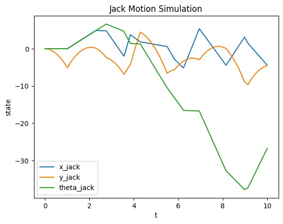
plt.plot(tvec, traj[3], label='x_jack')
plt.plot(tvec, traj[4], label='y_jack')
plt.plot(tvec, traj[5], label='theta_jack')
plt.title('Jack Motion Simulation')
plt.xlabel('t')
plt.ylabel('state')
plt.legend(loc="best")
plt.show()

Simulation Params

tspan = [0, 10]
dt = 0.01
s0 = np.array([...])  # 12-element state vector

Simulation time: $10$ seconds
Timestep: $\Delta t = 0.01$
Initial condition $s_0$ is the system at rest (all zero position and velocity)

A time vector is constructed with:

tvec = np.linspace(tspan[0], tspan[1], N)

Where:

N = \frac{t_{\text{final}} - t_{\text{start}}}{\Delta t}

Running the Simulation

traj = simulate_impact(dynamics, s0, tspan, dt, integrate)

Using the previously defineed function, we integrate the system forward in time using:

Continuous-time dynamics via dynamics()
Impact detection via impact_condition()
Post-impact update via impact_update()

The result traj is a $12 \times N$ matrix, where each row corresponds to one state variable over time.

Here are the results: schematic

Animation

Using the following function provided by my instructor, Prof. Todd Murphey, I animated the motion of the of the entire system, which is shown at the top of this page.

The code works as I expected (after a lot of debugging). Since the box rotates due to an external force, its impacts with the jack induce angular acceleration on the jack. Also, the force due to gravity does not accelerate the box downwards, since there is an equal constraint force holding the box up. However, over time, the box tends to drift downwards over time, since the jack is subject to gravity. However, if neither the jack nor the box were to be subject to gravity, then the average y position (long term) of the box would be 0, since the jack’s impacts would not be biased by the force of gravity.

def animate_jack_in_a_box(config_array,l=1,w=0.2,T=10):
    """
    Function to generate web-based animation of the system

    Parameters:
    ================================================
    config_array:
        trajectory of theta1 and theta2, should be a NumPy array with
        shape of (2,N)
    L1:
        length of the first pendulum
    L2:
        length of the second pendulum
    T:
        length/seconds of animation duration

    Returns: None
    """
    ################################
    # Imports required for animation. (leave this part)
    from plotly.offline import init_notebook_mode, iplot
    from IPython.display import display, HTML
    import plotly.graph_objects as go

    #######################
    # Browser configuration. (leave this part)
    def configure_plotly_browser_state():
        import IPython
        display(IPython.core.display.HTML('''
            <script src="/static/components/requirejs/require.js"></script>
            <script>
              requirejs.config({
                paths: {
                  base: '/static/base',
                  plotly: 'https://cdn.plot.ly/plotly-1.5.1.min.js?noext',
                },
              });
            </script>
            '''))
    configure_plotly_browser_state()
    init_notebook_mode(connected=False)


    ###############################################
    # Getting data from pendulum angle trajectories.
    N = len(config_array[0])

    x_box_array = config_array[0]
    y_box_array = config_array[1]
    theta_box_array = config_array[2]
    x_jack_array = config_array[3]
    y_jack_array = config_array[4]
    theta_jack_array = config_array[5]

    b1_x_array = np.zeros(N, dtype=np.float32)
    b1_y_array = np.zeros(N, dtype=np.float32)
    b2_x_array = np.zeros(N, dtype=np.float32)
    b2_y_array = np.zeros(N, dtype=np.float32)
    b3_x_array = np.zeros(N, dtype=np.float32)
    b3_y_array = np.zeros(N, dtype=np.float32)
    b4_x_array = np.zeros(N, dtype=np.float32)
    b4_y_array = np.zeros(N, dtype=np.float32)

    j_x_array = np.zeros(N, dtype=np.float32)
    j_y_array = np.zeros(N, dtype=np.float32)
    j1_x_array = np.zeros(N, dtype=np.float32)
    j1_y_array = np.zeros(N, dtype=np.float32)
    j2_x_array = np.zeros(N, dtype=np.float32)
    j2_y_array = np.zeros(N, dtype=np.float32)
    j3_x_array = np.zeros(N, dtype=np.float32)
    j3_y_array = np.zeros(N, dtype=np.float32)
    j4_x_array = np.zeros(N, dtype=np.float32)
    j4_y_array = np.zeros(N, dtype=np.float32)

    for t in range(N):
        g_w_b = get_se3_np(x_box_array[t], y_box_array[t], theta_box_array[t])
        g_w_j = get_se3_np(x_jack_array[t], y_jack_array[t], theta_jack_array[t])

        b1 = g_w_b.dot(np.array([l_box, l_box, 0, 1]))
        b1_x_array[t] = b1[0]
        b1_y_array[t] = b1[1]
        b2 = g_w_b.dot(np.array([l_box, -l_box, 0, 1]))
        b2_x_array[t] = b2[0]
        b2_y_array[t] = b2[1]
        b3 = g_w_b.dot(np.array([-l_box, -l_box, 0, 1]))
        b3_x_array[t] = b3[0]
        b3_y_array[t] = b3[1]
        b4 = g_w_b.dot(np.array([-l_box, l_box, 0, 1]))
        b4_x_array[t] = b4[0]
        b4_y_array[t] = b4[1]

        j = g_w_j.dot(np.array([0, 0, 0, 1]))
        j_x_array[t] = j[0]
        j_y_array[t] = j[1]
        j1 = g_w_j.dot(np.array([l_jack, 0, 0, 1]))
        j1_x_array[t] = j1[0]
        j1_y_array[t] = j1[1]
        j2 = g_w_j.dot(np.array([0, -l_jack, 0, 1]))
        j2_x_array[t] = j2[0]
        j2_y_array[t] = j2[1]
        j3 = g_w_j.dot(np.array([-l_jack, 0, 0, 1]))
        j3_x_array[t] = j3[0]
        j3_y_array[t] = j3[1]
        j4 = g_w_j.dot(np.array([0, l_jack, 0, 1]))
        j4_x_array[t] = j4[0]
        j4_y_array[t] = j4[1]

    ####################################
    # Axis limits.
    xm = -13
    xM = 13
    ym = -13
    yM = 13

    ###########################
    # Defining data dictionary.
    data=[dict(name = 'Box'),
          dict(name = 'Jack'),
          dict(name = 'Mass1_Jack'),
        ]

    ################################
    # Preparing simulation layout.
    layout=dict(xaxis=dict(range=[xm, xM], autorange=False, zeroline=False,dtick=1),
                yaxis=dict(range=[ym, yM], autorange=False, zeroline=False,scaleanchor = "x",dtick=1),
                title='Jack in a Box Simulation',
                hovermode='closest',
                updatemenus= [{'type': 'buttons',
                               'buttons': [{'label': 'Play','method': 'animate',
                                            'args': [None, {'frame': {'duration': T, 'redraw': False}}]},
                                           {'args': [[None], {'frame': {'duration': T, 'redraw': False}, 'mode': 'immediate',
                                            'transition': {'duration': 0}}],'label': 'Pause','method': 'animate'}
                                          ]
                              }]
               )

    ########################################
    # Defining the frames of the simulation.
    frames=[dict(data=[
            dict(x=[b1_x_array[k],b2_x_array[k],b3_x_array[k],b4_x_array[k],b1_x_array[k]],
                 y=[b1_y_array[k],b2_y_array[k],b3_y_array[k],b4_y_array[k],b1_y_array[k]],
                 mode='lines',
                 line=dict(color='red', width=3)
                 ),
            dict(x=[j1_x_array[k],j3_x_array[k],j_x_array[k],j2_x_array[k],j4_x_array[k]],
                 y=[j1_y_array[k],j3_y_array[k],j_y_array[k],j2_y_array[k],j4_y_array[k]],
                 mode='lines',
                 line=dict(color='blue', width=3)
                 ),
            go.Scatter(
                x=[j1_x_array[k],j2_x_array[k],j3_x_array[k],j4_x_array[k]],
                y=[j1_y_array[k],j2_y_array[k],j3_y_array[k],j4_y_array[k]],
                mode="markers",
                marker=dict(color='red', size=6)),
                 ]) for k in range(N)]

    #######################################
    # Putting it all together and plotting.
    figure1=dict(data=data, layout=layout, frames=frames)
    iplot(figure1)

#animate!
animate_jack_in_a_box(traj)

Jack-in-the-Box Lagrangian Mech. Simulation

Table of Contents

Simulation Output

Introduction

Imports

Santa’s Little Helper Functions

mat(g)

unhat(g)

get_se3_np(x, y, \theta)

integrate(f, x_t, dt, time)

simulate*impact(f, x_0, t∗spant*{\text{span}}t∗span, dt, integrate\text{integrate}integrate)

System Parameters, Transformations, and Lagrangian Derivation

Parameters

Generalized Coordinates

External Forces

Rigid Body Transforms

Rigid Body Velocities

Inertia Matrices

Lagrangian Formulation

Solving EL Equations

Numerical Integration of System Dynamics

Lambdified Acceleration Functions

Dynamics Function

Acceleration Matrix

Dummy Symbol Substitution

Impact Modeling with Constraints and Energy Conservation

Jack Pose Vector

Impact Constraints

Hamiltonian

Jacobian of Constraints

Impact Equations at τ⁺

Final Assembly of Equations

Impact Detection and Handling

Lambdifying the Constraint Function

Impact Detection Function

Variables for Post-Impact Velocities

Impact Update Function

Steps:

1. Substitution

2. Solve

3. Select Valid Solution

Output

Simulation

Simulation Params

Running the Simulation

Animation

simulateimpact(f, x_0, $t{\text{span}}$ , dt, $\text{integrate}$ )